Mohammed Billoo, founder of MAB Labs, provides custom embedded Linux solutions for a multitude of hardware platforms. In a series of posts over the coming weeks, he will walk us through the new Linux support in Tracealyzer v4.4, using a real-world project as an example.
 Recently, I’ve been working on a custom Linux driver to consume data streamed by an external device. While there are mechanisms native to the Linux kernel to ensure that the functionality of the driver is correct, evaluating performance is not straightforward. Percepio had recently announced a major update of the Tracealyzer support for Linux tracing (https://percepio.com/tz/tracealyzer-for-linux/) and released a public beta version, so it seemed like a good opportunity to try it out. Therefore I opted to use Tracealyzer for Linux to help me assess the performance of my custom driver and identify any deficiencies. This series of blog posts will demonstrate how to use Tracealyzer to evaluate the performance of a Linux kernel driver.
Tracealyzer for Linux takes advantage of LTTng, an open source tracer and profiler that allows developers to evaluate performance of the kernel (including drivers). It also supports userspace applications, but the focus of this series will be on the kernel. Ultimately, Tracealyzer parses the output of LTTng and provides visualization and detailed statistics to allow a developer to evaluate the performance of their kernel/driver.
To understand what we’re looking to accomplish, it’s important to diagram our driver:
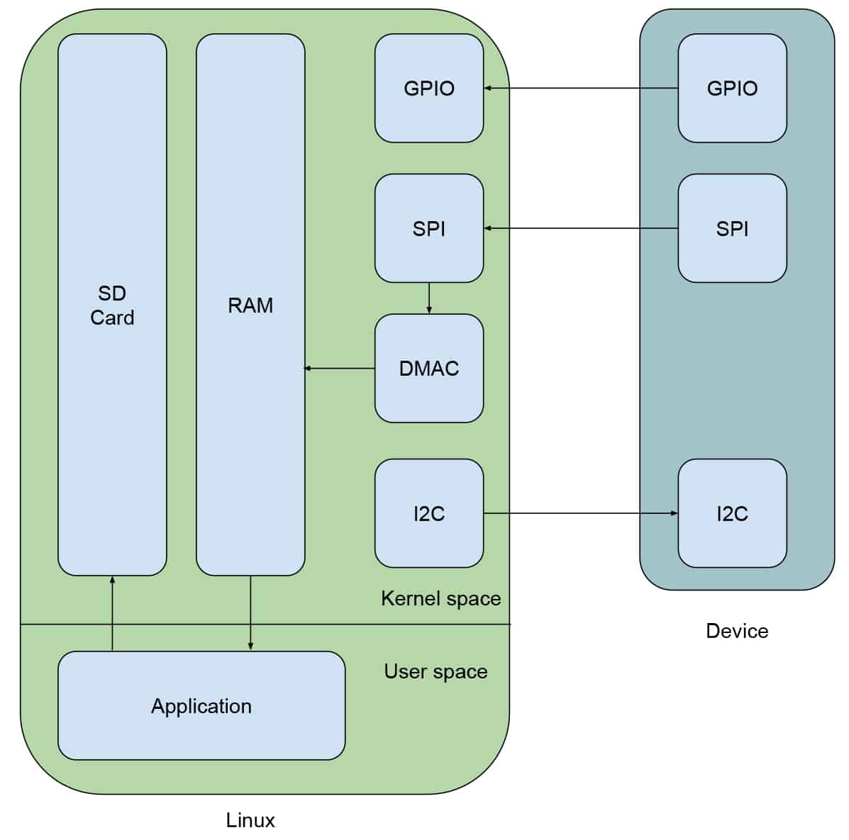
Our external device has three main interfaces. The I2C interface is meant to control the device, the SPI interface is used to stream data back to our Linux device, and the GPIO is an interrupt line to indicate when there is data ready to be consumed. When the GPIO line is asserted by our device, the Linux driver will send an I2C command to instruct the device to begin streaming, which will be done over the SPI interface. The driver will instruct the DMA controller (DMAC) of our embedded Linux system to manage the data transfer between the SPI bus and system RAM to ensure that the CPU is able to manage other tasks. While the driver will simply instruct the DMAC to perform the necessary transfers, it will need to periodically check in to make sure that there are no issues. Finally, application code exists on the Linux device to retrieve the streamed data from RAM and store it in non-volatile memory.
We’re going to leverage Tracealyzer to help us validate two important metrics. First, that the amount of time from the GPIO being asserted to when the I2C command is issued is kept to a minimum. Second, that the Linux kernel is providing the driver with sufficient execution cycles to allow it to periodically manage any issues encountered by the DMAC. Our ultimate goal is to guarantee that minimal data is lost in the streaming process, and Tracealyzer will help quantify this guarantee.
Configure the device development kit
As mentioned before, Tracealyzer leverages files generated by LTTng. Before getting started with any implementation, we need to first get our embedded Linux platform appropriately configured to support LTTng. The platform I selected was the Phytec i.MX 6ULL development kit. I’ve used other Phytec development kits in the past and am comfortable with their Yocto-based Board Support Package (BSP).
We’re going to have to customize the BSP to support LTTng, since the standard BSP for this board doesn’t include LTTng by default. To do this, we’re going to create our own layer that is on top of the “poky” layer and the custom Phytec layers. While a deeper discussion of the Yocto Project is outside of the scope of this article, don’t fret! You can follow along using my github repo.
Our custom layer is called “meta-mab-percepio” and its directory structure is as follows:
tree -d sources/meta-mab-percepio/
sources/meta-mab-percepio/
├── conf
├── recipes-images
   ├── images
   └── packagegroups
└── recipes-kernel
   └── linux
└── linux-mainline- conf consists of the layer configuration, which is a standard Yocto practice.
- recipes-images/packagegroups contains “packagegroup-custom.bb”, which is a file that contains that necessary LTTng packages that we will need in the resulting images.
- recipes-images/images/ contains “phytec-headless-image.bbappend”, which is our own customization to the Phytec Linux image. It simply adds the “packagegroup-custom” to the image.
- recipes-kernel/linux/ contains a recipe to add the necessary customization to the Linux kernel to support LTTng.
With the above customizations, we’ll be able to simply build the Linux image, load it on the SD card, boot it on the development kit, and run through the instructions on Percepio’s “Getting Started with Tracealyzer for Linux” page to collect the appropriate traces.
Once we’ve run the necessary commands outlined in the link above and have a directory called “lttng-traces” in the home directory of root, we can copy it over to our x86(_64) machine for analysis in Tracealyzer. This can be done by simply powering off the Phytec development kit, and copying the directory from the SD card over to the PC. Another way is to transfer the trace data over a network connection, Tracealyzer has integrated features for that.
The most important views at this stage
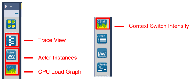
After we launch Tracealyzer, select “File->Open Folder” and select the “lttng-traces” directory. Tracealyzer will analyze the directory for the captured trace session and load all included files (an LTTng trace consists of multiple files). Then we can choose the appropriate view to analyze the performance of our driver. While Tracealyzer has views to provide useful insights into the userspace-kernel interaction, our focus is going to be in the kernel space and thus the “Trace View”, the “Actor Instances”, the “CPU Load Graph”, and the “Context Switch Intensity” views. These views can be selected by clicking on the appropriate icon on the left bar in the main Tracealyzer window:
If we open the Trace View, we are presented with the following graph:
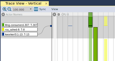
The leftmost column shows the “Actor Names”, which are the userspace and kernel processes/threads that are executing at any given time. The leftmost column (in gray) is the kernel “swapper” which is the idle task in the Linux kernel. If we move further right, we see the blue line, which is a kernel thread (“kworker”). As we implement the driver and monitor its performance using Tracealyzer, we’re going to use the Trace View to verify that our kernel thread is given enough execution resources to manage the DMA transfer. As we move even further to the right, we see the lttng userspace process in green, and finally the rcu_sched userspace process in yellow. A detailed account of rcu_sched is outside the scope of this article, but this article is a great starting point.
If we right click in the window and select “Zoom Out – Show Full Traces”, we are presented with this concise view of all the threads and processes that are executed during the entire duration of the capture:
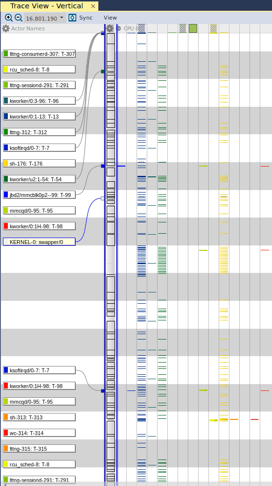
Here we see that the swapper is occupying the most execution resources during the entire capture. This makes sense, since we’re not actually doing any substantial task. When our driver is running and transferring data from our device to the Phytec development board, we should expect to see sections of the Trace View that are consumed by blue fragments. This would indicate that our specific kernel thread is given a greater chunk of the execution resources on the platform to perform the transfer.
The next important view is the “Actor Instances”, where we have selected the “Execution Time” in the drop down box at the top left:
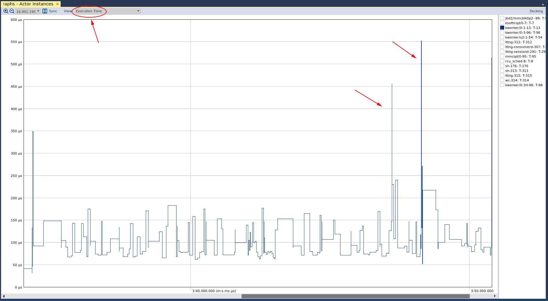
The y-axis of this graph indicates the amount of time that is being occupied by any particular “actor” (which is defined as any execution element, such as a thread or process). When we have one of the kernel threads selected, we can see that there are a few spikes in its execution time. We can also see that these spikes are approximately 350, 450, and 550 microseconds. To understand if these spikes are of any real concern, we would either need timing requirements of our system, or evaluate how the system operates under “normal” conditions. Since we don’t have any requirements, we have to infer whether these spikes are of real concern. We’ll use the next view to do just that. If we select another kernel thread, we see the following anomalous graph:
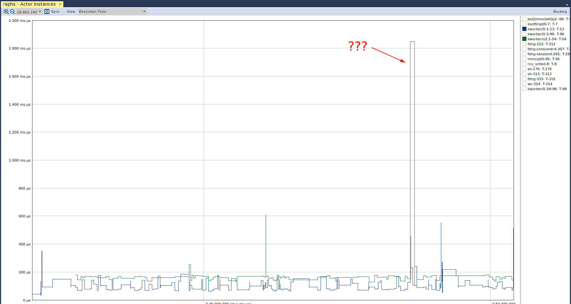
Here we see that there is a relatively large spike in the execution time of one of the kernel threads. Again, we’re going to use the next view to determine if this is cause for concern.
As mentioned, the next view is the “CPU Load”, which tells us the CPU utilization of different actors. If we open that view, we see the following graph:
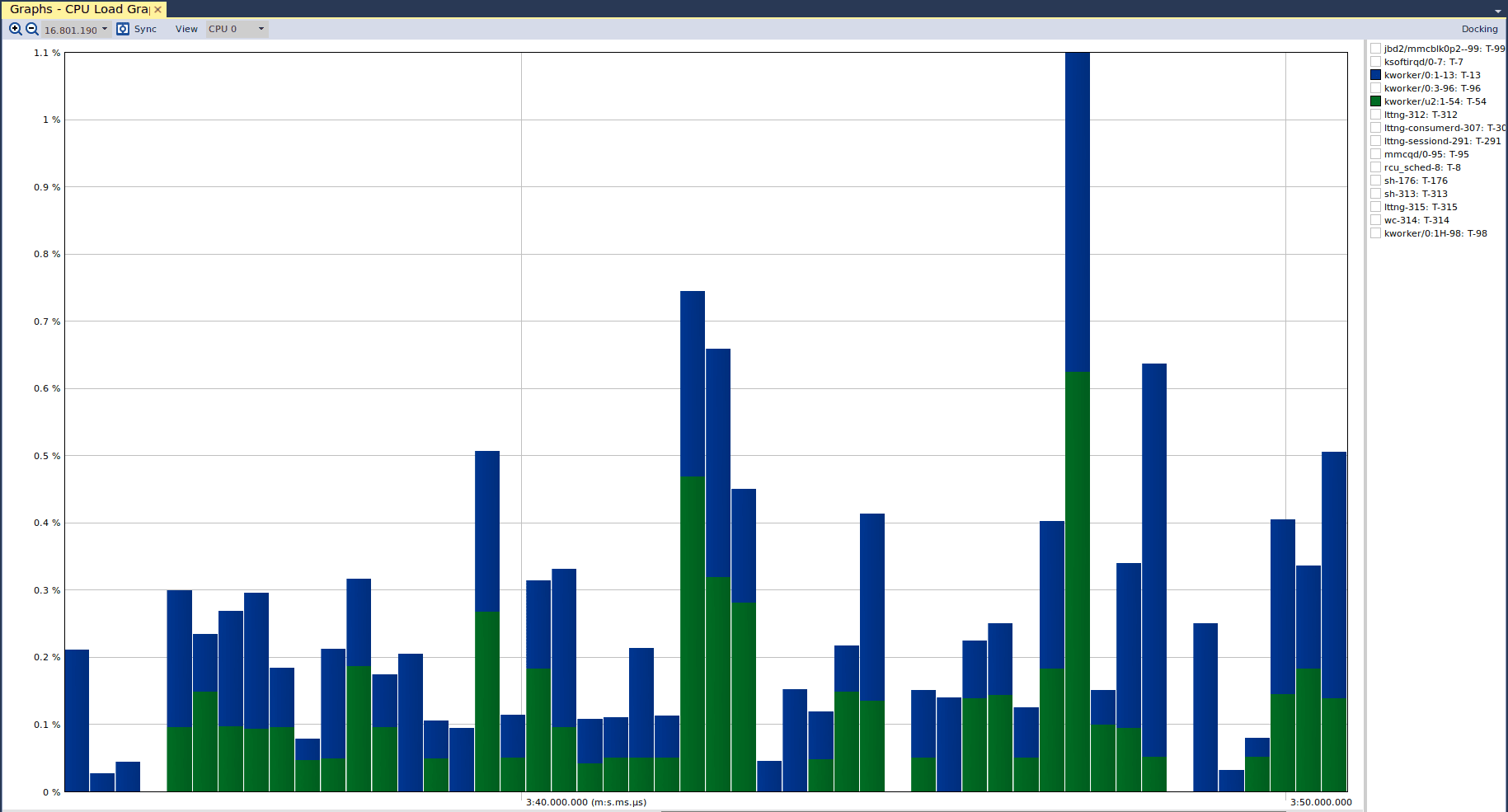 And we can see that there was no cause for concern. The CPU utilization for both kernel threads never exceeded 1.1%, and so what we saw in the “Actor Instance” graph was simply a spike in the execution time of the green kernel thread relative to the blue kernel thread. It is important to note that Tracealyzer defaults the y-axis to support visible presentation of the data, which is why we do not see the y-axis capped at 100% (we wouldn’t see much!) If we select the “lttng-sessiond” actor in the CPU load graph, we see the following:
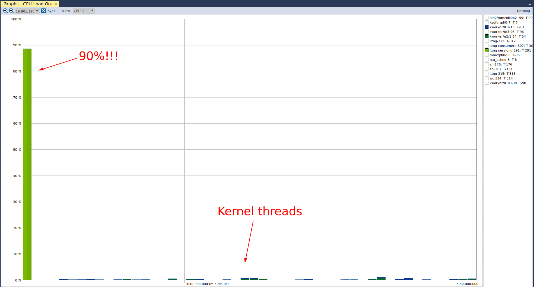
Here we see that the “lttng-sessiond” process occupies 90% of the CPU near the beginning of the trace (again, it’s important to note that Tracealyzer adjusted the y-axis to accommodate a meaningful view of the data). While this is substantial, this is expected since the lttng userspace daemon needs to perform the necessary initialization to capture traces. Moreover, there is not much else going on that competes for the CPU time. For comparison purposes, we can also see the CPU utilization of the kernel threads.
The final view is the “Context Switch Intensity” view, which allows us to validate that our kernel driver is performant and not causing the kernel to thrash. If we take a look at that view, we can see the following:
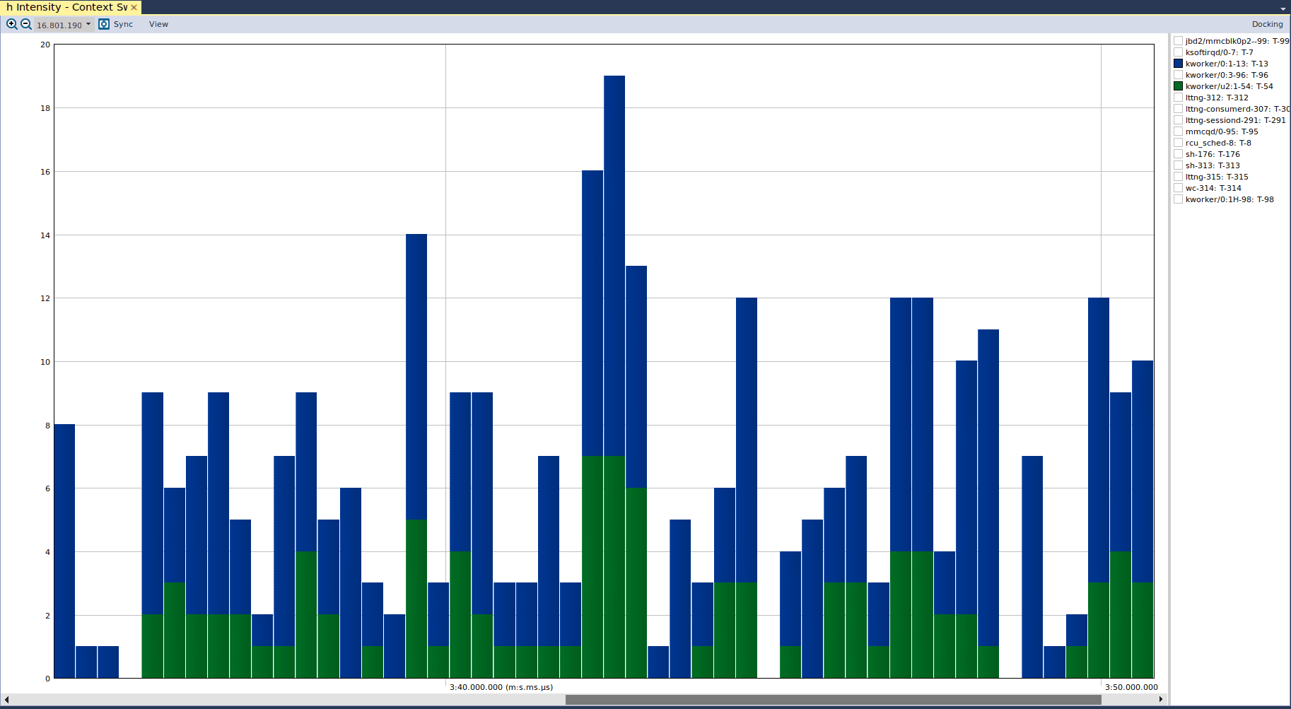
Here we see that there are not any significant context switches for any particular kernel thread, relative to others. If there were a performance issue in our driver, then we may see significant context switches of our kernel thread. This would be due to the kernel scheduler giving execution time to our kernel thread, then moving to another thread after some time, but then switching immediately back to our thread if it has demanded execution resources. Again, the determination of whether approximately 20 context switches – as shown in the above graph – is acceptable is dependent either on the system requirements or on measurements performed when the system is behaving “normally”.
These views also provide a quick way to overview the trace and locate “hotspots” or anomalies of interest for further study, especially if you don´t know exactly what to look for. This is one of the main benefits of Tracealyzer, as they otherwise can be difficult to find in long traces with many thousands or even millions of events.
In summary, Tracealyzer provides numerous valuable perspectives of the execution of our driver. Each perspective provides a unique insight into the perspective of the Linux system, including the kernel. When combined, these perspectives should be used to give us a holistic view of our driver to ensure that there are no performance bottlenecks, or allow us to identify the cause of any bottlenecks for us to investigate further. As follow-ups, we’ll begin building up our driver and continue to use Tracealyzer to validate its performance.
Mohammed Billoo, MAB Labs
This is the first in a series of articles about using Tracealyzer to capture and analyze visual trace diagnostics for embedded Linux systems.