
The use of Real-Time Operating System (RTOS) is increasingly common in embedded software designs, as an RTOS makes it easy to divide your code into smaller blocks, tasks, which execute seemingly in parallel and independent of each other. An RTOS provides multi-tasking, in a reliable and maintainable manner, which makes it easier to design applications with multiple concurrent functions such as control, communication and HMI. The overhead of an RTOS is negligible on modern 32-bit processors and is often more than compensated for by more efficient designs enabled by multi-tasking. At the center of this multi-tasking model is the RTOS scheduler — the part of the kernel responsible for deciding which task runs at any given moment. Understanding how it works, and how to read the timing data it produces, is essential once you move from “the code compiles” to “the system meets its deadlines”.
RTOS Scheduling and Fixed-Priority Multitasking
An RTOS typically implements preemptive multi-tasking using a periodic interrupt routine (the “tick” interrupt) that switches the running task when required. The decision of what task to execute is known as task scheduling and most RTOS use fixed-priority scheduling (FPS), where the developers assign each task a static priority level to indicate their relative urgency. The RTOS scheduler always chooses the task with highest priority from the tasks currently ready to execute. This is a quite simple and elegant solution that allows the RTOS scheduler to be very small, highly optimized and thoroughly validated.
In fixed-priority preemptive scheduling, that tick interrupt evaluates whether a higher-priority task has become ready; if so, the current task is immediately preempted. It is however important to assign suitable task priorities, otherwise the system performance will suffer or the system might even become unresponsive. This is because high priority tasks may prevent lower priority tasks from executing if they consume too much processor time. Analyzing task priorities and runtime behavior of RTOS-based applications requires recording and visualization of the task scheduling. For this purpose Percepio offers the Tracealyzer tools with over 25 interactive views that make the recorded traces easier to comprehend and analyze.
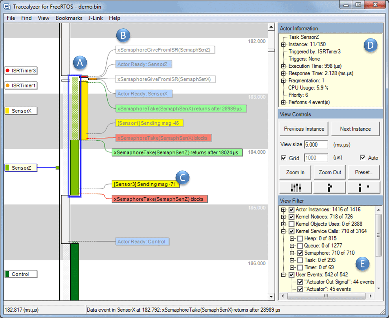
Figure 1: Tracealyzer showing RTOS task scheduling and calls to RTOS services.
Figure 1 shows the main view of Tracealyzer, a vertical timeline focused on the execution of tasks and interrupt handlers (A) annotated with text labels showing events (B) including RTOS API calls and custom “user events” (C). The “Actor Information” panel (D) shows properties of the highlighted task and the “View Filter” (E) allows for filtering of the display. Double-clicking on task fragments or event labels opens other related views showing related points in the trace, e.g., a chronological list of all executions of a selected task.
Execution Time vs. Response Time
A critical distinction to understand in RTOS scheduling is execution time versus response time. Execution time is the actual CPU time a task consumes. Response time is the total elapsed time from task activation to completion — which includes all preemptions by higher-priority tasks and ISRs. A task with a long response time is not necessarily a slow task; it may simply be one that is repeatedly interrupted by higher-priority work. The response time of a task, i.e., the time from activation until completion, is affected not just by the actual processor time used by the task itself (execution time), but also by higher priority tasks and interrupts that preempt the task, as illustrated in Figure 1. So if the response time is too long, optimizing the code of the problematic task might be a waste of time, unless you know what actually causes the long response time. In one traced example, a task’s peak execution time was 1,087 µs — but its peak response time reached 3,255 µs. The difference was caused entirely by interference from other tasks and interrupts, not by the task’s own code. Identifying the true cause requires RTOS-aware analysis, not just per-task profiling.
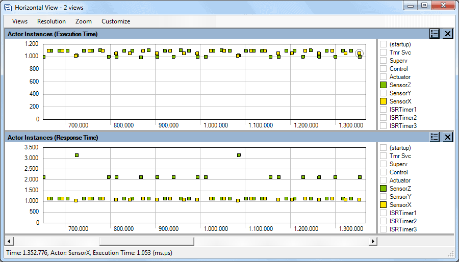
Figure 2: Execution time and response time for each execution of two tasks.
With Tracealyzer you get many perspectives of the runtime world, including plots of task execution times and response times like in Figure 2. We can see that execution times are pretty steady for both tasks, but sometimes the response time of “SensorZ” is much higher. By clicking on such a data point, you open the corresponding interval in the main trace view (Figure 1) and see the cause. All 25+ views in Tracealyzer are interconnected in similar ways.
Standard program-counter sampling profilers give only an aggregate picture of execution time and miss sporadic overruns that cause real problems. RTOS-aware tracing records the full sequence of scheduler events, ISR activations, and kernel object operations, and can present execution time and response time as time-series plots and histograms — making it straightforward to identify whether a timing problem is caused by the task itself or by interference from higher-priority work.
Want to learn more about RTOS-based development and Tracealyzer? Read more articles here!