This is a part of Tracealyzer Hands On, a series of blog posts with use-case examples for Percepio Tracealyzer®.
During the last few posts, we have been exploring how to setup user events and state machines and how we can analyze such traces. In this post, we are going to examine how developers can configure the trace view better suit their particular system and the analysis at hand, and fit more information into the available screen space.
The trace view is a set of “view fields”, where the leftmost field (CPU 0) shows the thread execution trace. Each actor (task, thread or interrupt) has one swimlane each, and are typically sorted by scheduling priority. Important events like kernel calls are displayed as floating labels in the rightmost field (“Event Field”), although not currently showing any event labels due to the zoom level and filter settings.
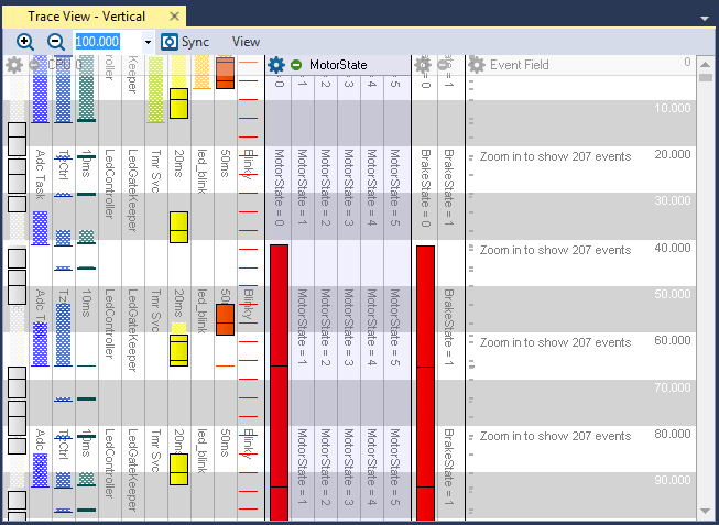
View fields can be added, closed, rearranged, collapsed, expanded and configured individually. An example can be seen in the image above, where we have added two additional view fields for showing state machines, “MotorState” and “BrakeState”.
View fields can be collapsed using the green minus sign which makes more room for other fields. A collapsed field is not hidden, but is displayed as single column (or row) that takes minimal space.
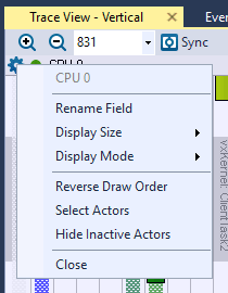
Under the gear icon you find a menu with several options for customizing the particular view field, as shown above. For example, this menu allows developers to:
- Rename the field
- Change the included information (e.g. what tasks to show)
- Change display options, depending on the type of field (e.g. the width of task columns)
- Close the field
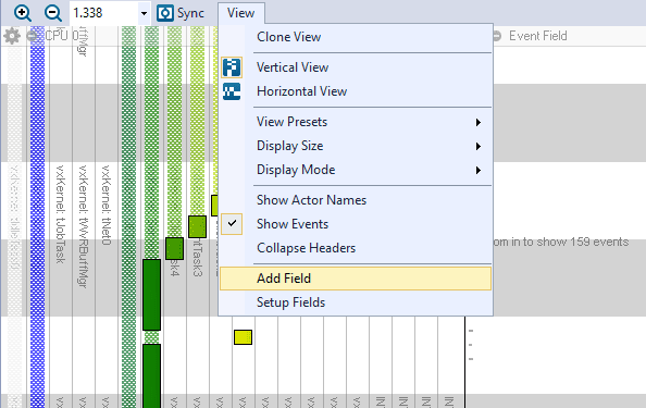
Additional fields can by added by selecting “Add Field”, found under “View” in the trace view menu, as shown below. In this menu you also find “Setup Fields”, where you can modify all field settings and even reorder the fields, if you like.
When selecting “Add Field”, the following dialog is shown, where you select what type of view field to add.
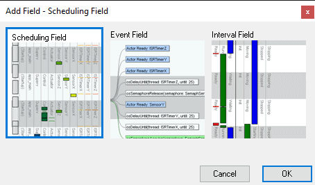
Currently there are three types of view fields:
- Scheduling field: task and ISR trace
- Event field: event labels, like kernel API calls and User Events, and the hot-spot indication
- Interval field: intervals and state machines
The scheduling field has several configuration options, including:
- Changing the display mode (Gantt, compact, merged)
- Reversing the draw order
- Hide Inactive Actors
- Actor selection
The display mode can be changed between the standard Gantt view (one column per actor), a compact view (a single column), or a merged view. The merged view is more compact than the Gantt view by stacking the actors based on preemptions, which tends to reveal hotspots in the trace.
Reversing the draw order allows you to change the order in which tasks are drawn. By default, Tracealyzer orders the actors based on scheduling priority, with the lowest priority task on the left (or in the bottom, when using the horizontal orientation), but you can swap the order if you prefer.
The Hide Inactive Actors option compresses the scheduling field when using Gannt mode by hiding the actor columns that are currently empty. Scrolling or zooming automatically changes what columns that are hidden, with a small delay to avoid flickering. This is not enabled by default, but Tracealyzer will ask you about using this feature when motivated by the content and window size.
 The actor selection is worthwhile to discuss in a bit more detail. This option allows a developer to selectively decide which tasks and interrupts will be displayed in a particular scheduling field. For example, let’s say that we are debugging an issue with a system that has 15 tasks, but the issue is related to only a few of these. Then we can deselect these other actors and only display the tasks of relevance to the current debug session.
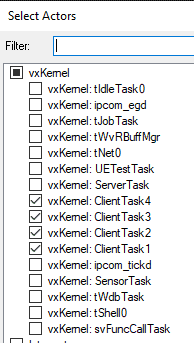
In order to do this, you click the gear and then press “Select Actors” which open a pop-up window similar to what you see to the right here. Select the desired tasks and interrupts and proceed; only the checked actors will be displayed in the scheduling field. Note that this filtering is independent from the main filter, normally found in the bottom right corner.
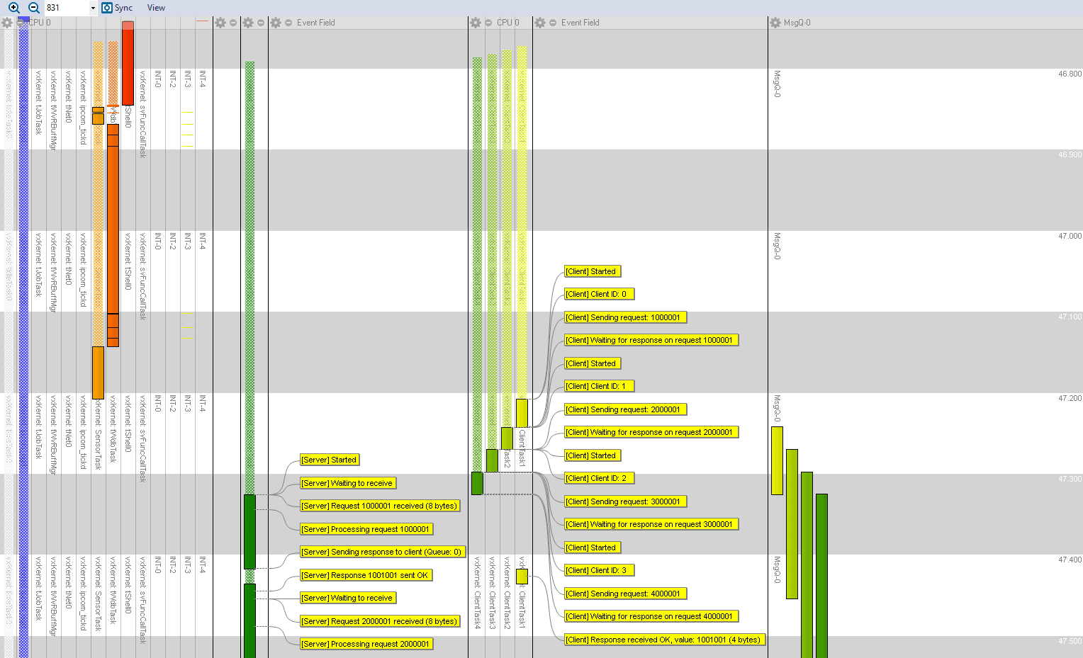
An interesting capability is that you can create several view fields of the same type, but with different settings and selections. This allows you to separate the trace into multiple fields, based on what you are interested in. In the below example, we have divided the tasks into three groups by creating two additional scheduling fields and the “Select Actor” option. We have also added two additional event fields, one for each scheduling field, which lets us show more event labels in the available screen space. Moreover, to the far right there also an Interval field, showing the messages in a message queue.
Event fields do not offer much options, as they are automatically connected to the Scheduling fields on their left side. In the above example, each scheduling field has its own event field, but you can let several scheduling fields share a single event field if desired. Just make sure that the Event field(s) are placed on the right of the desired Scheduling fields. You change the field order using the View -> Setup Field dialog.
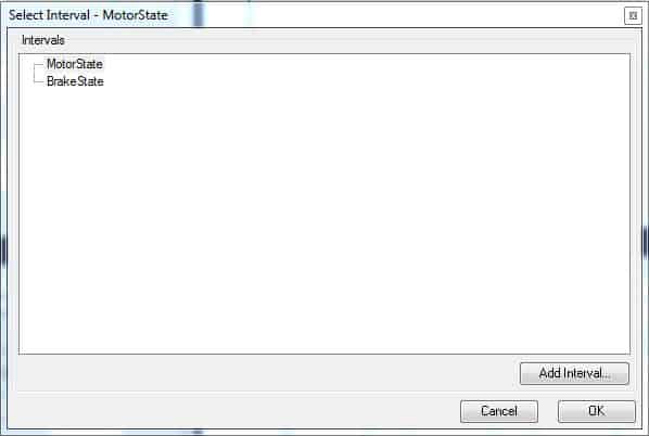
When adding Interval fields, like the message queue in the above example, you get to select a data set to display, i.e. an interval or a state machine. Previously defined intervals and state machines are listed in the Select Interval screen, as shown below. Moreover, the “Add Interval…” button allows you to select from pre-defined intervals and state machines that Tracealyzer is aware of automatically, such as the message queue in the above example. You can change the displayed data set later if you like, using the “Select Interval” option in the View menu.
Finally, a short note regarding vertical and horizontal trace orientation. The new trace view allows for both vertical and horizontal orientation of the time line, with identical functionality. Both modes have their advantages, so now you can use all capabilities also in horizontal mode. Moreover, you can easily switch the orientation of your current trace window as you please, using the options “Vertical View” and “Horizontal View” found in the View menu. An example of the horizontal orientation is shown below.

As we have seen throughout this post, the view fields allow a developer to easily customize which actors and data it is that they want to see in their trace. This provides the ability to make a view cleaner and to get at the most interesting or relevant data without any distractions or unnecessary actors crowding the view.